Potential class

This class defines an atomistic potential to be used by Pysic. An interaction between two or more particles can be defined and the targets of the interaction can be specified by chemical symbol, tag, or index. The available types of potentials are always inquired from the Fortran core to ensure that any changes made to the core are automatically reflected in the Python interface.

There are a number of utility functions in pysic for inquiring the keywords and other data needed for creating the potentials. For example:

• Inquire the names of available potentials: list_valid_potentials()
• Inquire the names of parameters for a potential: names_of_parameters()
• Ask for a short description of a potential: description_of_potential()

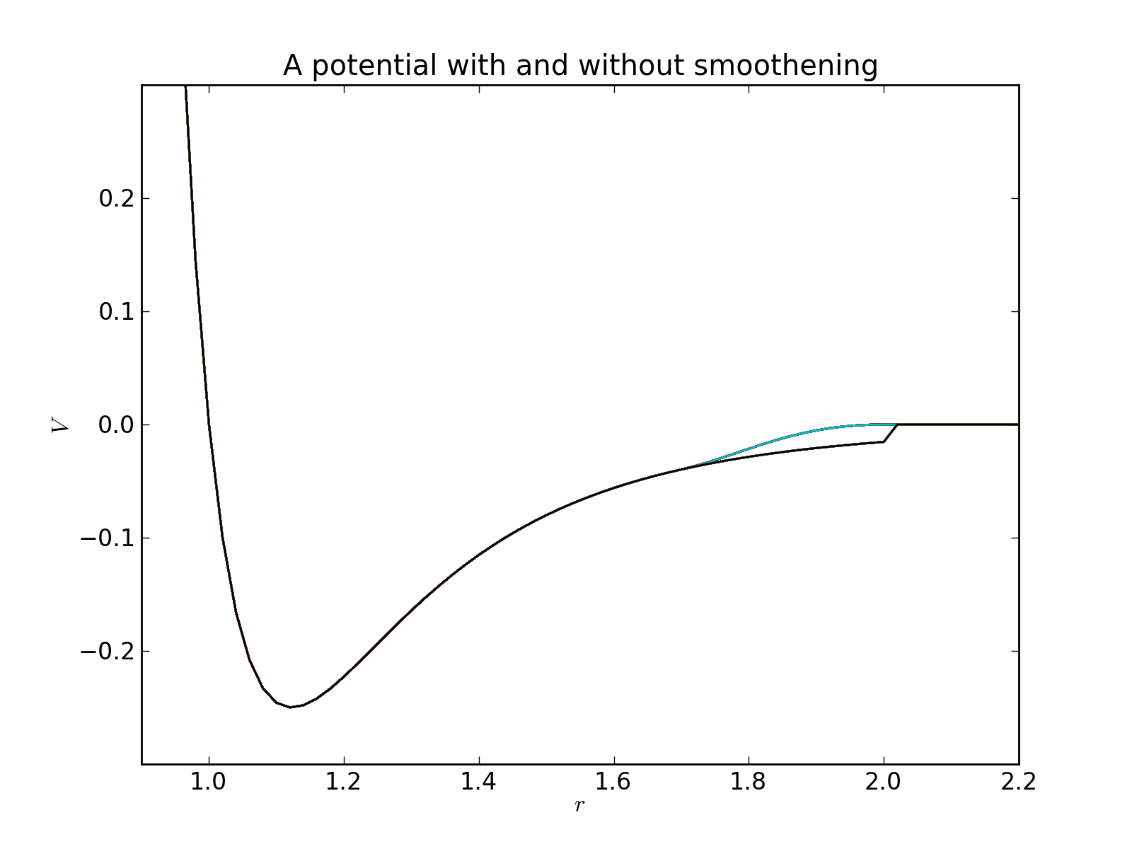
Cutoffs

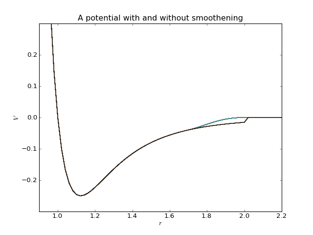
Many potentials decay towards zero in infinity, but in a numeric simulation they are cut at a finite range as specified by a cutoff radius. However, if the potential is not exactly zero at this range, a discontinuity will be introduced. It is possible to avoid this by including a smoothening factor in the potential to force a decay to zero in a finite interval:

\[\tilde{V}(r) = f(r) V(r),\]

where the smoothening factor is (for example)

\[\begin{split}f(r) = \begin{cases} 1, & r < r_\mathrm{soft} \\ \frac{1}{2}\left(1+\cos \pi\frac{r-r_\mathrm{soft}}{r_\mathrm{hard}-r_\mathrm{soft}}\right), & r_\mathrm{soft} < r < r_\mathrm{hard} \\ 0, & r > r_\mathrm{hard} \end{cases}.\end{split}\]

Pysic allows one to specify both a hard and a soft cutoff for all potentials to include such a smooth cutoff. If no soft cutoff if given or it is zero (or equal to the hard cutoff), no smoothening is applied.

[hires.png, pdf]

Targets of a Potential

A Potential needs targets to describe interactions. For instance a 2-body potential needs two targets. These targets can be specified as chemical species (through the corresponding chemical symbols), indices, or tags (as defined in ASE Atoms). The most typical use is by symbols.

The targets need to be specified as lists. For example, if one wishes to define a Potential affecting He-He pairs, it can be defined through:

>>> pot = Potential(...)
>>> pot.set_symbols(['He','He'])

There are also utility functions for generating these lists more conveniently from strings: pysic.utility.convenience.expand_symbols_string() and pysic.utility.convenience.expand_symbols_table(). For example:

>>> from pysic.utility.convencience import expand_symbols_string as sym
>>> from pysic.utility.convencience import expand_symbols_table as tab
>>> print sym('HeHe')
[['He', 'He']]
>>> print tab(sym('Si,SiO'))
[['Si', 'Si'], ['Si', 'O']]

List of currently available potentials

Below is a list of potentials currently implemented. Also see the List of corrently available compound potentials.

• Constant potential
• Constant force potential
• Charge self energy potential
• Power decay potential
• Shifted power potential
• Harmonic potential
• Lennard-Jones potential
• Buckingham potential
• Exponential potential
• Charged-pair potential
• Absolute charged-pair potential
• Charge dependent exponential potential
• Tabulated potential
• Bond bending potential
• Dihedral angle potential

Constant potential

1-body potential defined as

\[V(\mathbf{r}) = V,\]

i.e., a constant potential.

A constant potential is of course irrelevant in force calculation since the gradient is zero. However, one can add a BondOrderParameters bond order factor with the potential to create essentially a bond order potential.

The constant potential can also be used for assigning an energy offset which depends on the number of atoms of required types.

Keywords:

>>> names_of_parameters('constant')
['V']

Fortran routines:

• create_potential_characterizer_constant_potential()
• evaluate_energy_constant_potential()

Constant force potential

1-body potential defined as

\[V(\mathbf{r}) = - \mathbf{F} \cdot \mathbf{r},\]

i.e., a constant force \(\mathbf{F}\).

Keywords:

>>> names_of_parameters('force')
['Fx', 'Fy', 'Fz']

Fortran routines:

• create_potential_characterizer_constant_force()
• evaluate_energy_constant_force()
• evaluate_force_constant_force()

Charge self energy potential

1-body potential defined as

\[V(q) = \varepsilon q^n,\]

where \(\varepsilon\) is an energy scale constant and \(n\) an integer exponent. Note that only the integer part of the exponent is taken if a real number is given. This is because you must expect negative values for \(q\) and so a non-integer \(n\) would be ill-defined.

Keywords:

>>> names_of_parameters('charge_self')
['epsilon', 'n']

Fortran routines:

• create_potential_characterizer_constant_force()
• evaluate_energy_constant_force()
• evaluate_force_constant_force()

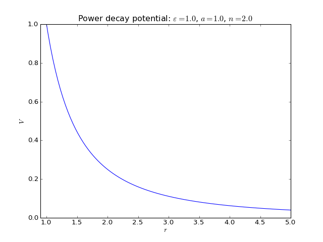
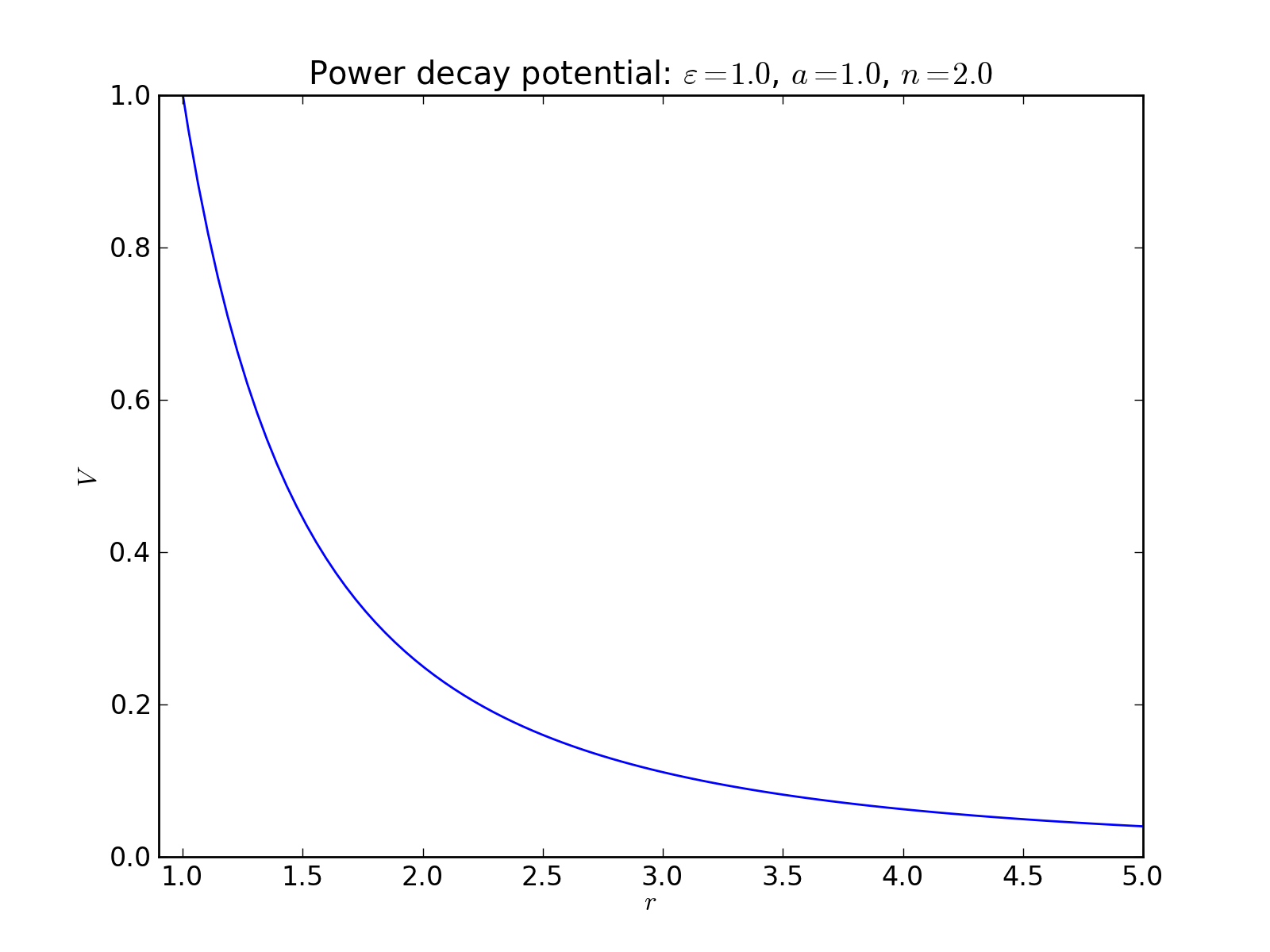
Power decay potential

2-body interaction defined as

\[V(r) = \varepsilon \left( \frac{a}{r} \right)^n\]

where \(\varepsilon\) is an energy scale constant, \(a\) is a lenght scale constant or lattice parameter, and \(n\) is an exponent.

There are many potentials defined in Pysic which already incorporate power law terms, and so this potential is often not needed. Still, one can build, for instance, the Lennard-Jones potential potential by stacking two power decay potentials. Note that \(n\) should be large enough fo the potential to be sensible. Especially if one is creating a Coulomb potential with \(n = 1\), one should not define the potential through Potential objects, which are directly summed, but with the CoulombSummation class instead.

Keywords:

>>> names_of_parameters('power')
['epsilon', 'a', 'n']

[hires.png, pdf]

Fortran routines:

• create_potential_characterizer_power()
• evaluate_energy_power()
• evaluate_force_power()

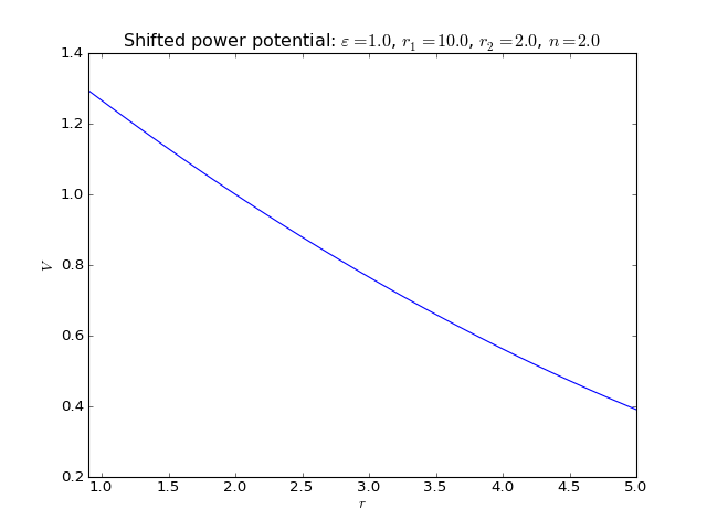
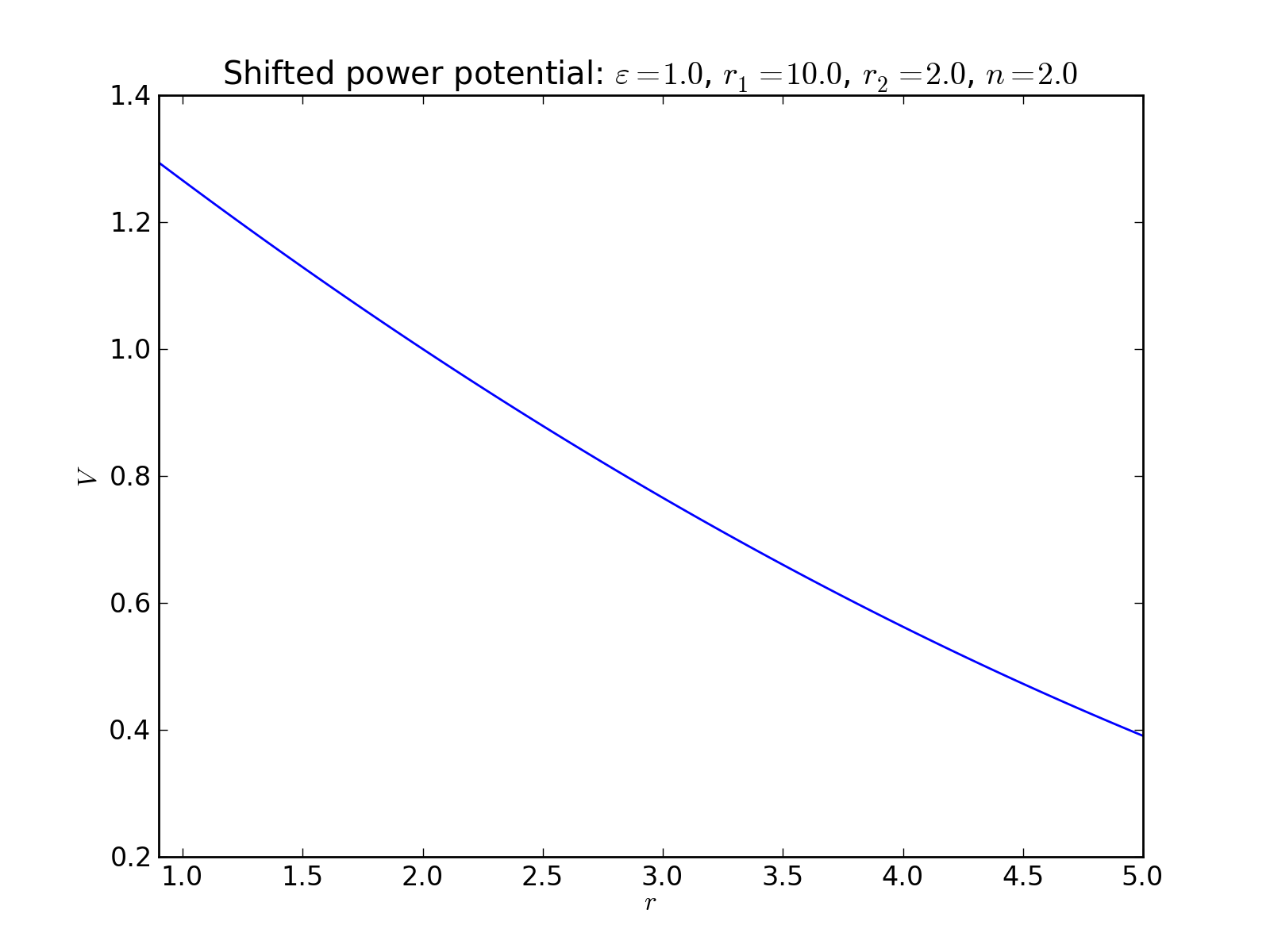
Shifted power potential

2-body interaction defined as

\[V(r) = \varepsilon \left( \frac{r_1 - r}{r_1 - r_2} \right)^n\]

where \(\varepsilon\) is an energy scale constant, \(r_1\) and \(r_2\) are a lenght scale constants, and \(n\) is an exponent.

Keywords:

>>> names_of_parameters('shift_power')
['epsilon', 'r1', 'r2', 'n']

[hires.png, pdf]

Fortran routines:

• create_potential_characterizer_shift()
• evaluate_energy_shift()
• evaluate_force_shift()

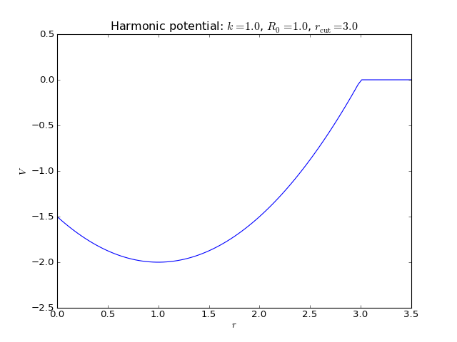
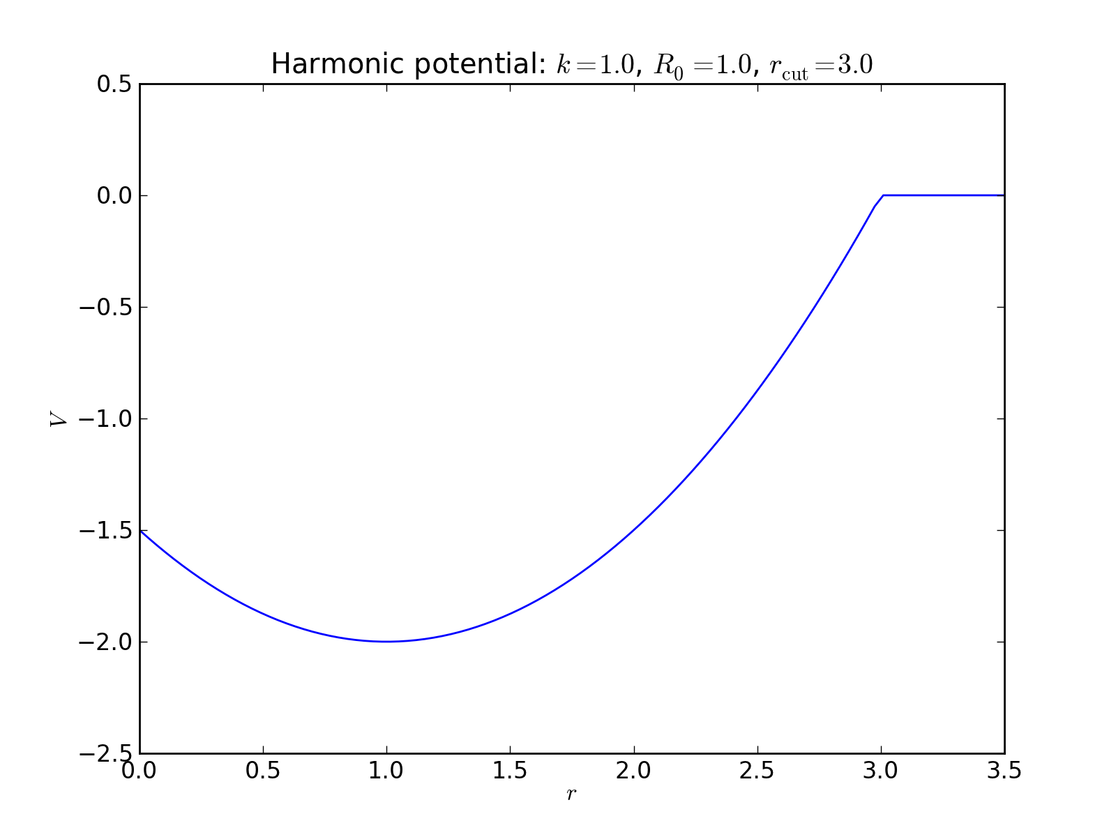
Harmonic potential

2-body interaction defined as

\[V(r) = \frac{1}{2} k (r-R_0)^{2} - \frac{1}{2} k (r_\mathrm{cut}-R_0)^2,\]

where \(k\) is a spring constant, \(R_0\) is the equilibrium distance, and \(r_\mathrm{cut}\) is the potential cutoff. The latter term is a constant whose purpose is to remove the discontinuity at cutoff.

Keywords:

>>> names_of_parameters('spring')
['k', 'R_0']

[hires.png, pdf]

Fortran routines:

• create_potential_characterizer_spring()
• evaluate_energy_spring()
• evaluate_force_spring()

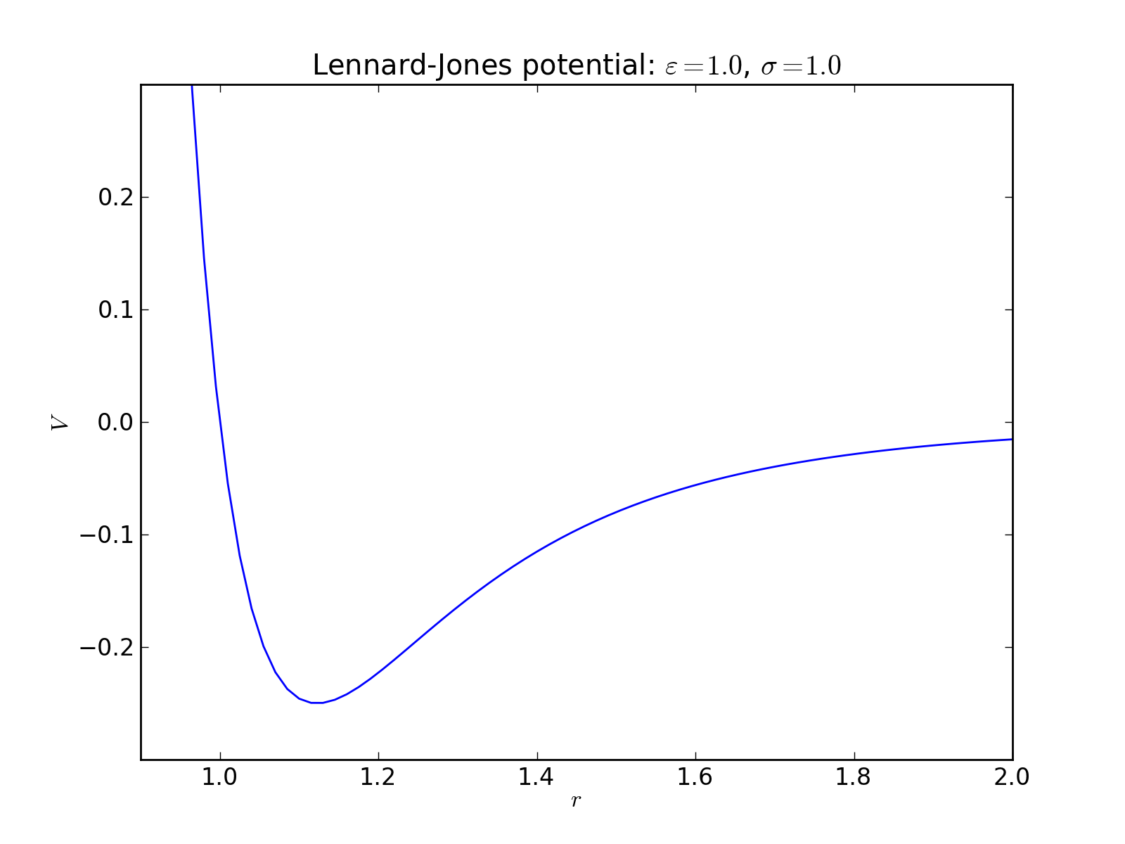
Lennard-Jones potential

2-body interaction defined as

\[V(r) = \varepsilon \left[ \left( \frac{\sigma}{r} \right)^{12} - \left( \frac{\sigma}{r} \right)^{6} \right],\]

where \(\varepsilon\) is an energy constant defining the depth of the potential well and \(\sigma\) is the distance where the potential changes from positive to negative in the repulsive region.

Keywords:

>>> names_of_parameters('LJ')
['epsilon', 'sigma']

[hires.png, pdf]

Fortran routines:

• create_potential_characterizer_LJ()
• evaluate_energy_LJ()
• evaluate_force_LJ()

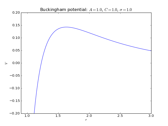
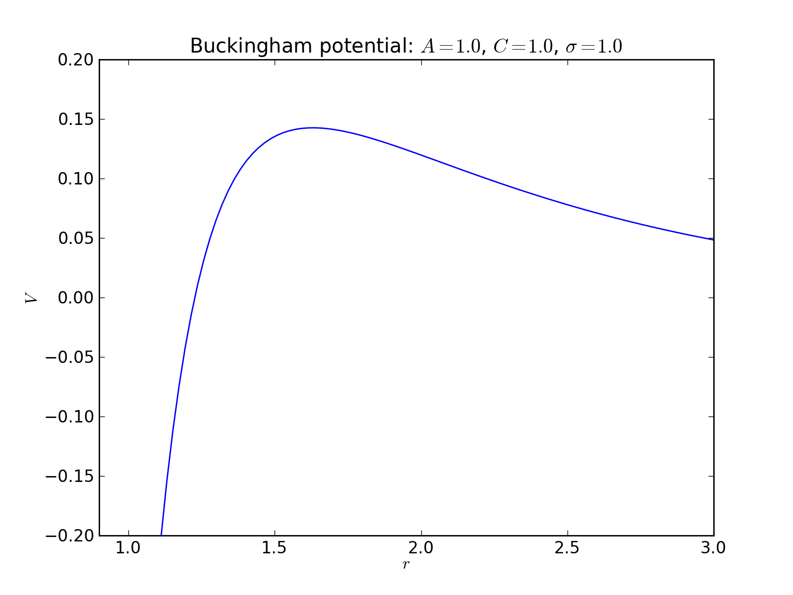
Buckingham potential

2-body interaction defined as

\[V(r) = A e^{-\frac{r}{\sigma}} - C \left( \frac{\sigma}{r} \right)^6\]

where \(\sigma\) is a length scale constant, and \(A\) and \(C\) are the energy scale constants for the exponential and van der Waals parts, respectively.

Keywords:

>>> names_of_parameters('Buckingham')
['A', 'C', 'sigma']

[hires.png, pdf]

Fortran routines:

• create_potential_characterizer_buckingham()
• evaluate_energy_buckingham()
• evaluate_force_buckingham()

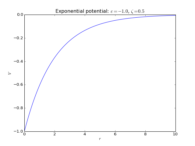
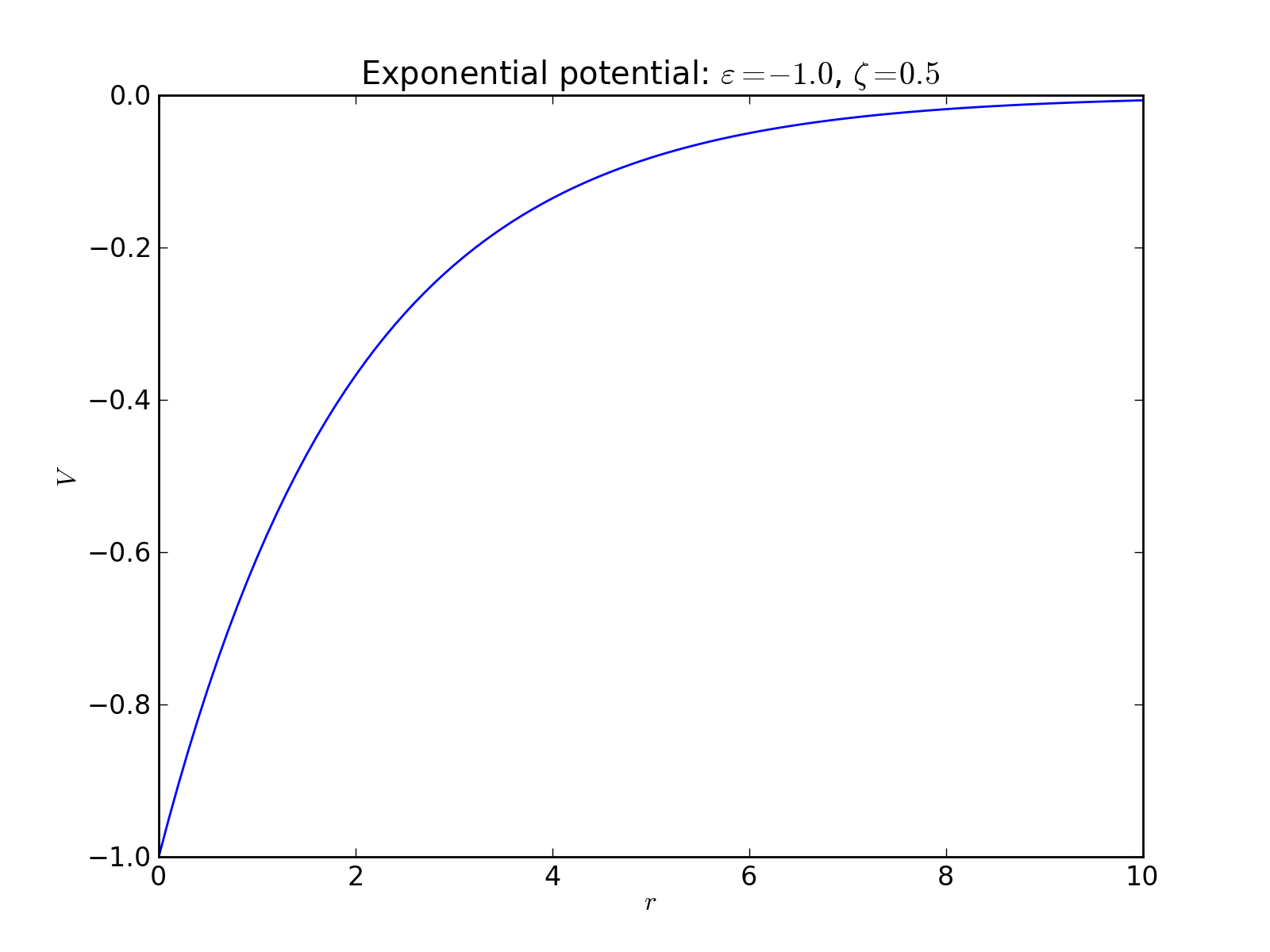
Exponential potential

2-body interaction defined as

\[\begin{split}V(q) & = \varepsilon \exp(-\zeta r)\end{split}\]

where \(\varepsilon\) is an energy scale constant and \(\zeta\) is a length decay constant.

Keywords:

>>> names_of_parameters('exponential')
['epsilon', 'zeta']

[hires.png, pdf]

Fortran routines:

• create_potential_characterizer_exp()
• evaluate_energy_exp()
• evaluate_force_exp()

Charged-pair potential

2-body interaction defined as

\[V(q_1,q_2) = \varepsilon q_1^{n_1} q_2^{n_2}\]

where \(\varepsilon\) is an energy scale constant, and \(n_i\) are integer exponents.

This potential is similar to the Charge self energy potential, but it affects two atoms. It is mainly meant to be used together with distance dependent potentials in a ProductPotential to add charge dependence to other potentials. For instance:

pot1 = pysic.Potential('power')
pot2 = pysic.Potential('charge_pair')
prod = pysic.ProductPotential([pot1,pot2])

Defines the potential

\[V(q_1,q_2,r) = \varepsilon q_1^{n_1} q_2^{n_2} \left(\frac{a}{r}\right)^n\]

Keywords:

>>> names_of_parameters('charge_pair')
['epsilon', 'n1', 'n2']

Fortran routines:

• create_potential_characterizer_charge_pair()
• evaluate_energy_charge_pair()
• evaluate_electronegativity_charge_pair()

Absolute charged-pair potential

2-body interaction defined as

\[\begin{split}V(q_1,q_2) & = \sqrt{ B_1(q_1) B_2(q_2) }\\ B_i(q_i) & = a_i + b_i | q_i - Q_i |^{n_i}\end{split}\]

where \(a_i\) is an energy shift, \(b_i\) is a scale constant, \(Q_i\) is a charge shift, and \(n_i\) are real exponents.

This potential is similar to the Charged-pair potential, but it affects the absolute values of charges. This allows one to use real valued exponents instead of just integers. Note though, that the product \(B_1(q_1) B_2(q_2)\) must be positive for all relevant values of \(q_i\).

Keywords:

>>> names_of_parameters('charge_abs')
['a1', 'b1', 'Q1', 'n1',
 'a2', 'b2', 'Q2', 'n2']

Fortran routines:

• create_potential_characterizer_charge_pair_abs()
• evaluate_energy_charge_pair_abs()
• evaluate_electronegativity_charge_pair_abs()

Charge dependent exponential potential

2-body interaction defined as

\[\begin{split}V(q) & = \varepsilon_{ij} \exp\left(\frac{\xi_i D_i(q_i) + \xi_j D_j(q_j)}{2} \right) \\ D_i(q) & = R_{i,\max} + | \beta_i (Q_{i,\max} - q) |^{\eta_i} \\ \beta_i & = \frac{ (R_{i,\min} - R_{i,\max})^\frac{1}{\eta_i} }{ Q_{i,\max} - Q_{i,\min} }\\ \eta_i & = \frac{ \ln \frac{R_{i,\max}}{R_{i,\max} - R_{i,\min}} }{ \ln \frac{Q_{i,\max}}{Q_{i,\max} - Q_{i,\min}} },\end{split}\]

where \(\varepsilon\) is an energy scale constant, \(\xi_i\) are charge decay constants, and \(R_{i,\min/\max}\) and \(Q_{i,\min/\max}\) are the changes in valence radii and charge, respectively, of the ions for the minimum and maximum charge. \(D_i(q)\) is the effective atomic radius for the charge \(q\).

Keywords:

>>> names_of_parameters('charge_exp')
['epsilon',
 'Rmax1', 'Rmin1', 'Qmax1', 'Qmin1',
 'Rmax2', 'Rmin2', 'Qmax2', 'Qmin2',
 'xi1', 'xi2']

Fortran routines:

• create_potential_characterizer_charge_exp()
• evaluate_energy_charge_exp()
• evaluate_electronegativity_charge_exp()

Tabulated potential

2-body interaction of the type \(V(r)\) defined with a tabulated list of values.

The values of the potential are read from text files of the format:

V(0)     V'(0)*R
V(dr)    V'(dr)*R
V(2*dr)  V'(2*dr)*R
...      ...
V(R)     V'(R)*R

where V and V' are the numberic values of the potential and its derivative (\(V(r)\) and \(V'(r)\)), respectively, for the given values of atomic separation \(r\). The grid is assumed to be uniform and starting from 0, so that the values of \(r\) are \(0, \mathrm{d}r, 2\mathrm{d}r, \ldots, R\), where \(R\) is the range of the tabulation and \(\mathrm{d}r = R/(n-1)\) where \(n\) is the number of value pairs (lines) in the table. Note that the first and last derivatives are forced to be zero regardless of what is given in the table (\(V'(0) = V'(R) = 0\)).

For each interval \([r_i,r_{i+1}]\) the value of the potential is calculated using third degree spline (cspline) interpolation

\[\begin{split}r \in & [r_i,r_{i+1}]: \\ t(r) = & \frac{r-r_i}{r_{i+1}-r_i} \\ V(r) = & V(r_i) h_{00}(t) + V'(r_i) (r_{i+1}-r_i) h_{10}(t) + \\ & V(r_{i+1}) h_{01}(t) + V'(r_{i+1}) (r_{i+1}-r_i) h_{11}(t) \\ h_{00}(t) = & 2t^3-3t^2+1 \\ h_{10}(t) = & t^3-2t^2+t \\ h_{01}(t) = & -2t^3+3t^2 \\ h_{11}(t) = & t^3-t^2\end{split}\]

The range of the tabulation \(R\) is given as a parameter when creating the potential. The tabulated values should be given in a text file with the name table_xxxx.txt, where xxxx is an identification integer with leading zeros (e.g., table_0001.txt). The id is also given as a parameter when defining the potential.

The tabulation range \(R\) is not the same as a cutoff. It merely defines the value of \(r\) for the last given value in the table. If the cutoff is longer than that, then \(V(r) = V(R)\) for all \(r > R\). If the cutoff is shorter than the range, then as for all potentials, \(V(r) = 0\) for all \(r > r_{\mathrm{cut}}\). A smooth cutoff (see Cutoffs) can also be applied on top of the tabulation. The reason for this formalism is that once you have tabulated your potential, you may change the cutoff and smoothening marginal without having to retabulate the potential.

You can also scale the potential in \(r\)-axis just by changing the range \(R\), which is the reason why the table needs to include the derivatives multiplied by \(R\): Say you tabulate a potential for a given \(R\), obtaining values \(V(r), V'(r)R\). If you scale the \(r\)-axis of the potential by a factor \(\rho\), \(R^* = \rho R\), you obtain a new potential \(U(r)\). This new potential is a scaling of the original potential \(U(r) = V(r/\rho), U'(r) = V'(r/\rho)/\rho\). The tabulated \(r\) values are scaled so that the \(i\)th value becomes \(r^*_i = \rho r_i\), and so the expected tabulated values are for the potential \(U(r_i^*) = V(r_i^*/\rho) = V(r_i)\) and for the derivative \(U'(r^*_i)R^* = V'(r^*_i/\rho)R^*/\rho = V'(r_i)R\). That is, the tabulated values are invariant under the scaling of \(R\).

Finally, another parameter is available for scaling the energy scale \(V(r) \to \varepsilon V(r)\).

The file containing the tabulated values is directly read in by the Fortran core, and it is not allowed to contain anything besides two equally long columns of real numbers separated by white spaces.

Keywords:

>>> names_of_parameters('tabulated')
['id', 'range', 'scale']

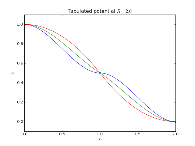
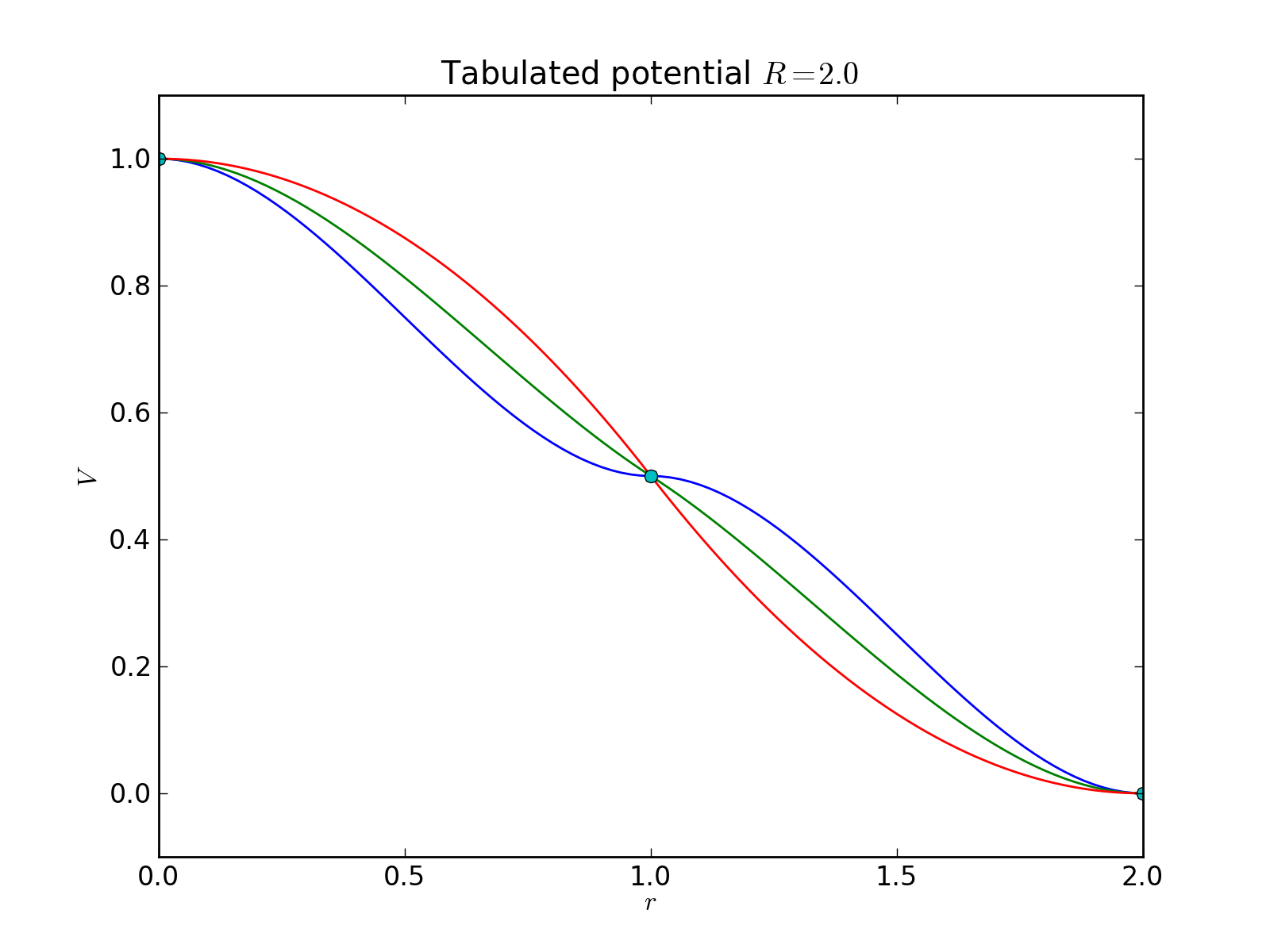
The example plot below shows the resulting potentials for table:

1.0  0.0
0.5  0.0
0.0  0.0

as well as similar tables with the second number on the second row replaced by -1.0 or -2.0 with range \(R=2.0\) (i.e., the midpoint gets derivative values of 0.0, -0.5, or -1.0).

[hires.png, pdf]

Fortran routines:

• create_potential_characterizer_table()
• evaluate_energy_table()
• evaluate_force_table()

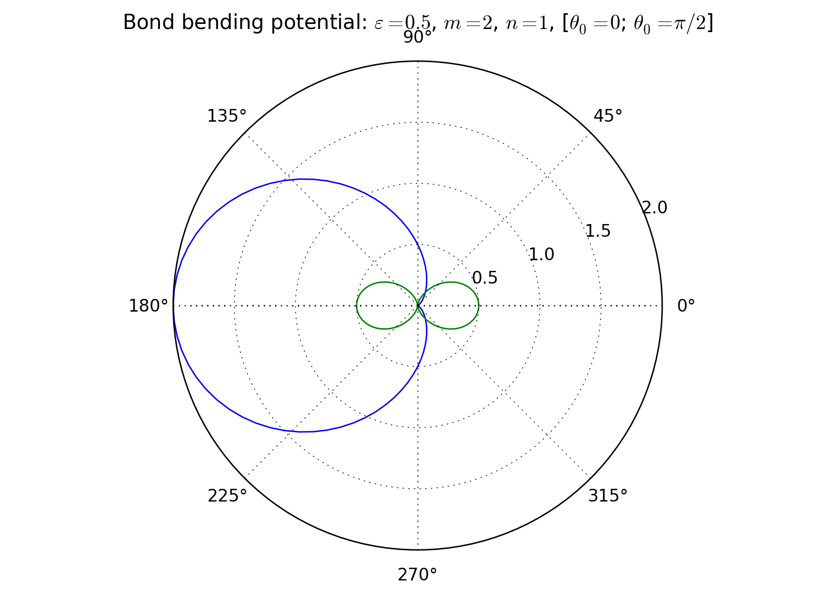
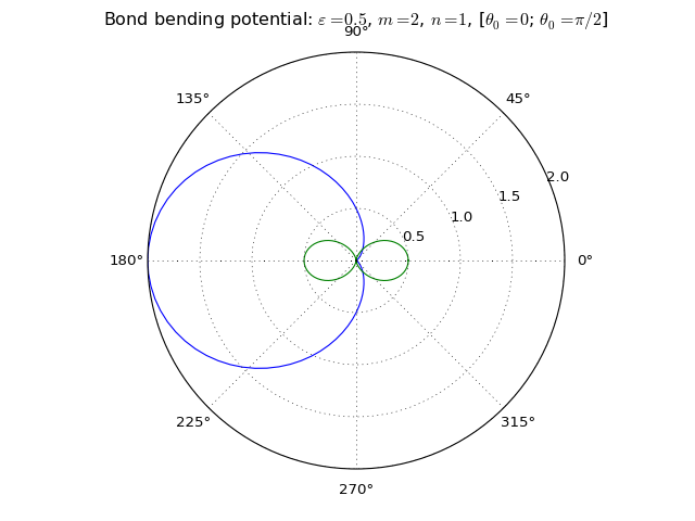
Bond bending potential

3-body interaction defined as

\[V(\theta) = \varepsilon ( \cos^n \theta - \cos^n \theta_0 )^m,\]

where \(\varepsilon\) is an energy scale constant, \(n\) and \(m\) are integer exponents, \(\theta\) is an angle defined by three points in space (atomic positions) and \(\theta_0\) is the equilibrium angle. As a apecial case, the cosine harmonic potential is obtined with \(\varepsilon = k/2, n=1, m=2\).

Keywords:

>>> names_of_parameters('bond_bend')
['epsilon', 'theta_0', 'n', 'm']

Three bodies form a triangle and so there are three possible angles the potential could bend. To remove this ambiguousness, the angle is defined so that as the potential is given a list of targets, the middle target is considered to be at the tip of the angle.

Example:

>>> pot = Potential('bond_bend')
>>> pot.set_symbols(['H', 'O', 'H'])

This creates a potential for H-O-H angles, but not for H-H-O angles.

Also remember that the bond bending potential does not include any actual bonding potential between particles - it only generates an angular force component. It must be coupled with other potentials to build a full bonding potential.

[hires.png, pdf]

Fortran routines:

• create_potential_characterizer_bond_bending()
• evaluate_energy_bond_bending()
• evaluate_force_bond_bending()

Dihedral angle potential

4-body interaction defined as

\[V(r) = \frac{k}{2} (\cos \theta - \cos \theta_0)^2\]

where \(k\) is a spring constant and \(\theta\) is the dihedral angle, with \(\theta_0\) denoting the equilibrium angle. (So, this is the cosine harmonic variant of the dihedral angle potential.)

For an atom chain 1-2-3-4 the dihedral angle is the angle between the bonds 1-2 and 3-4 when projected on the plane perpendicular to the bond 2-3. In other words, it is the torsion angle of the bond chain. If we write \(\mathbf{r}_{ij} = \mathbf{R}_j - \mathbf{R}_i\), where \(\mathbf{R}_i\) is the coordinate vector of the atom \(i\), the angle is given by

\[\begin{split}\cos \theta =& \frac{\mathbf{p} \cdot \mathbf{p}'}{|\mathbf{p}||\mathbf{p}'|}\\ \mathbf{p} =& -\mathbf{r}_{12} + \frac{\mathbf{r}_{12} \cdot \mathbf{r}_{23}}{|\mathbf{r}_{23}|^2}\mathbf{r}_{23}\\ \mathbf{p}' =& \mathbf{r}_{34} - \frac{\mathbf{r}_{34} \cdot \mathbf{r}_{23}}{|\mathbf{r}_{23}|^2}\mathbf{r}_{23}\end{split}\]

Keywords:

>>> names_of_parameters('dihedral')
['k', 'theta_0']

Fortran routines:

• create_potential_characterizer_dihedral()
• evaluate_energy_dihedral()
• evaluate_force_dihedral()

List of methods

Below is a list of methods in Potential, grouped according to the type of functionality.

Interaction handling

• get_cutoff()
• get_cutoff_margin()
• get_number_of_parameters()
• get_parameter_names()
• get_parameter_value()
• get_parameter_values()
• get_potential_type()
• get_soft_cutoff()
• set_cutoff()
• set_cutoff_margin()
• set_parameter_value()
• set_parameter_values()
• set_soft_cutoff()

Coordinator handling

• get_coordinator()
• set_coordinator()

Target handling

• accepts_target_list()
• add_indices()
• add_symbols()
• add_tags()
• get_different_indices()
• get_different_symbols()
• get_different_tags()
• get_indices()
• get_number_of_targets()
• get_symbols()
• get_tags()
• set_indices()
• set_symbols()
• set_tags()

Description

• describe()
• is_multiplier() (meant for internal use)
• get_potentials() (meant for internal use)

Full documentation of the Potential class

class pysic.interactions.local.Potential(potential_type, symbols=None, tags=None, indices=None, parameters=None, cutoff=0.0, cutoff_margin=0.0, coordinator=None)

Class for representing a potential.

Several types of potentials can be defined by specifying the type of the potential as a keyword. The potentials contain a host of parameters and information on what types of particles they act on. To view a list of available potentials, use the method list_valid_potentials().

A potential may be a pair or many-body potential: here, the bodies a potential acts on are called targets. Thus specifying the number of targets of a potential also determines if the potential is a many-body potential.

A potential may be defined for atom types or specifically for certain atoms. These are specified by the symbols, tags, and indices. Each of these should be either ‘None’ or a list of lists of n values where n is the number of targets. For example, if:

indices = [[0, 1], [1, 2], [2, 3]]

the potential will be applied between atoms 0 and 1, 1 and 2, and 2 and 3.

Parameters:

symbols: list of string

the chemical symbols (elements) on which the potential acts

tags: integer

atoms with specific tags on which the potential acts

indices: list of integers

atoms with specific indices on which the potential acts

potential_type: string

a keyword specifying the type of the potential

parameters: list of doubles

a list of parameters for characterizing the potential; their meaning depends on the type of potential

cutoff: double

the maximum atomic separation at which the potential is applied

cutoff_margin: double

the margin in which the potential is smoothly truncated to zero

coordinator: Coordinator object

the coordinator defining a bond order factor for scaling the potential

accepts_target_list(targets)

Tests whether a list is suitable as a list of targets, i.e., symbols, tags, or indices and returns True or False accordingly.

A list of targets should be of the format:

targets = [[a, b], [c, d]]

where the length of the sublists must equal the number of targets.

It is not tested that the values contained in the list are valid.

Parameters:

targets: list of strings or integers

a list whose format is checked

add_indices(indices)

Adds the given indices to the list of indices.

Parameters:

indices: list of integers

list of additional indices on which the potential acts

add_symbols(symbols)

Adds the given symbols to the list of symbols.

Parameters:

symbols: list of strings

list of additional symbols on which the potential acts

add_tags(tags)

Adds the given tags to the list of tags.

Parameters:

tags: list of integers

list of additional tags on which the potential acts

describe()

Prints a short description of the potential using the method describe_potential().

get_coordinator()

Returns the Coordinator.

get_cutoff()

Returns the cutoff.

get_cutoff_margin()

Returns the margin for a smooth cutoff.

get_different_indices()

Returns a list containing each index the potential affects once.

get_different_symbols()

Returns a list containing each symbol the potential affects once.

get_different_tags()

Returns a list containing each tag the potential affects once.

get_indices()

Return a list of indices on which the potential acts on.

get_number_of_parameters()

Return the number of parameters the potential expects.

get_number_of_targets()

Returns the number of targets.

get_parameter_names()

Returns a list of the names of the parameters of the potential.

get_parameter_value(param_name)

Returns the value of the given parameter.

Parameters:

param_name: string

name of the parameter

get_parameter_values()

Returns a list containing the current parameter values of the potential.

get_potential_type()

Returns the keyword specifying the type of the potential.

get_potentials()

Returns a list containing the potential itself.

This is a method ensuring cross compatibility with the ProductPotential class.

get_soft_cutoff()

Returns the lower limit for a smooth cutoff.

get_symbols()

Return a list of the chemical symbols (elements) on which the potential acts on.

get_tags()

Return the tags on which the potential acts on.

is_multiplier()

Returns a list containing False.

This is a method ensuring cross compatibility with the ProductPotential class.

set_coordinator(coordinator)

Sets a new Coordinator.

Parameters:

coordinator: a Coordinator object

the Coordinator

set_cutoff(cutoff)

Sets the cutoff to a given value.

This method affects the hard cutoff. For a detailed explanation on how to define a soft cutoff, see set_cutoff_margin().

Parameters:

cutoff: double

new cutoff for the potential

set_cutoff_margin(margin)

Sets the margin for smooth cutoff to a given value.

Many potentials decay towards zero in infinity, but in a numeric simulation they are cut at a finite range as specified by the cutoff radius. If the potential is not exactly zero at this range, a discontinuity will be introduced. It is possible to avoid this by including a smoothening factor in the potential to force a decay to zero in a finite interval.

This method defines the decay interval \(r_\mathrm{hard}-r_\mathrm{soft}\). Note that if the soft cutoff value is made smaller than 0 or larger than the hard cutoff value an InvalidPotentialError is raised.

Parameters:

margin: double

The new cutoff margin

set_indices(indices)

Sets the list of indices to equal the given list.

Parameters:

indices: list of integers

list of integers on which the potential acts

set_parameter_value(parameter_name, value)

Sets a given parameter to the desired value.

Parameters:

parameter_name: string

name of the parameter

value: double

the new value of the parameter

set_parameter_values(values)

Sets the numeric values of all parameters.

Parameters:

values: list of doubles

list of values to be assigned to parameters

set_parameters(values)

Sets the numeric values of all parameters.

Equivalent to set_parameter_values().

Parameters:

values: list of doubles

list of values to be assigned to parameters

set_soft_cutoff(cutoff)

Sets the soft cutoff to a given value.

For a detailed explanation on the meaning of a soft cutoff, see set_cutoff_margin(). Note that actually the cutoff margin is recorded, so changing the hard cutoff (see set_cutoff()) will also affect the soft cutoff.

Parameters:

cutoff: double

The new soft cutoff

set_symbols(symbols)

Sets the list of symbols to equal the given list.

Parameters:

symbols: list of strings

list of element symbols on which the potential acts

set_tags(tags)

Sets the list of tags to equal the given list.

Parameters:

tags: list of integers

list of tags on which the potential acts